
Between 15 and 20 July 2026, an intense and prolonged storm produced persistent rainfall from Atacama to Ñuble, with an especially anomalous signal in Atacama and Coquimbo. The storm was reinforced by a strong El Niño event, an atmospheric river connected to the tropical Pacific, and atmospheric conditions favourable for storm development (CR2, 2026; Meteored, 2026).
This post quantifies the event in terms of intensity, accumulation, critical duration and return period, and links that hydrometeorological signal with the impacts reported by SENAPRED, MOP, DGA, SNA and the mining sector.
1. How extreme was the rainfall in different parts of Chile?
In 72 hours, the preliminary early-access version of the ERA5-Land climate dataset estimated about 214 mm of rainfall in a grid cell in the Limarí Valley, Coquimbo, and about 160 mm in Punitaqui, only 90 km farther south. Both precipitation accumulations are of the same order of magnitude; however, their degree of exceptionality is very different. In Punitaqui, the frequency analysis based on Soto-Escobar et al. (2026) estimates a 101-year return period (T) for this event. In Limarí, by contrast, the event exceeded a 500-year return period. The calculated return period values do not represent an exact number of years until the event repeats. Rather, they indicate that, on average over the available statistics, an event of that magnitude is expected to be exceeded once every T years; the larger the calculated return period, the more extreme the analysed event. Typical design return periods for drainage works range from 2 to 500 years, depending on the importance of the infrastructure, the tolerable risk of failure and the estimated service life (Minvu, 2026; MOP, 2025).
The contrast between those two return periods summarizes the central idea of this post: rainfall amount alone is not enough to determine how exceptional a storm will be. A large accumulation can be relatively common in a wet climate, while a smaller amount can be extraordinarily high in an arid area. Exceptionality depends not only on the total millimetres accumulated, but also on event duration and local climatology.
A previous CR2 analysis described the meteorological configuration of the storm (CR2, 2026). Here we address several pending hydrological questions:
- How anomalous was the rainfall that occurred between Atacama and Ñuble?
- Which storm duration made this event genuinely exceptional?
- What can we say about this extreme event relative to precipitation behaviour during the historical period 1981-2021?
2. How did we measure how anomalous or improbable this event was?
To answer this question, we analysed maximum precipitation using moving windows of 6, 12, 24, 48 and 72 hours, applied to hourly data from the preliminary ERA5-Land product. For each grid cell and each duration, we calculated the maximum accumulated precipitation observed during the episode. We then expressed these values as mean intensities by dividing the accumulation by the corresponding duration.
This distinction matters. Accumulation is the total precipitation depth recorded during a time window and is expressed in millimetres. Mean intensity is that same accumulation divided by the window duration and is expressed in millimetres per hour. A short episode can have very high intensity and still accumulate less precipitation than a moderate-intensity event that persists for several days.
We then compared the maximum intensities obtained for each duration with the intensity-duration-frequency (IDF) curves corresponding to each grid cell. These curves were built from the ERA5-Land annual-maximum series for the 1981-2021 period, which spans 41 years, by fitting a stationary Gumbel extreme-value distribution following the methodology of Soto-Escobar et al. (2026) .
The statistical rarity of each intensity is expressed through its return period, T. For example, T = 100 years indicates that, under the fitted probabilistic model and assuming stationary conditions, an intensity of that magnitude or higher has an annual exceedance probability close to 1 %. This does not mean that the event occurs regularly once every hundred years, nor that its occurrence resets a waiting interval of one hundred years. Events of that magnitude can occur in consecutive years or remain unobserved for much longer periods.
The calculations were performed for each cell of the bias-corrected ERA5-Land product, with a spatial resolution of 0.1 degrees, equivalent to roughly 11 km at the equator. This resolution makes it possible to characterize regional patterns and compare the episode’s severity spatially, but it does not replace pluviograph observations and does not fully represent orographic gradients, convective cells or other sub-grid hydrometeorological processes.
The resulting values should therefore be interpreted as spatially consistent estimates for regional hydrometeorological diagnosis and comparison, not as exact measurements of precipitation at a point location.
3. How much, where and how intensely did it rain?
Figure 1 shows that one of the most relevant features of this storm was its persistence, together with a marked spatial shift in the maxima as the analysed duration increases. For a 6-hour window, the largest accumulation in the study area was located in the Limarí Valley, near Ovalle, with about 61 mm, equivalent to a mean intensity of 10.2 mm/h. As the time window expands, the maxima shift progressively toward Andean sectors, reaching around 143 mm in the most intense 24 hours and approximately 288 mm in the 72-hour window. In other words, short-duration maxima were mainly concentrated in valley sectors, while the largest long-duration accumulations were located toward the mountains.
Figure 1 also shows how maximum mean intensity changes across the five durations considered. Each panel represents, for each grid cell, the continuous window with the largest accumulated precipitation for a given duration, expressed as mean intensity in millimetres per hour. The common scale allows direct comparison of intensities between panels.
As expected, maximum mean intensities decrease as the window duration increases, because the strongest precipitation pulses are averaged within progressively longer intervals. As a result, the areas associated with the highest intensities shrink and the spatial field becomes more homogeneous. This duration dependence is particularly relevant from the perspective of hydrology and infrastructure design: urban drainage systems or culverts respond mainly to intense short-duration precipitation, while larger catchments, rivers and reservoirs integrate precipitation accumulated over several hours or even several days.
Figure 1 also shows an important result for interpreting event severity: the zones with the largest absolute intensities do not necessarily coincide with those where the largest return periods are estimated. In particular, inland sectors of Atacama show relatively low intensities, but they can correspond to statistically very infrequent events because of the local precipitation climatology.
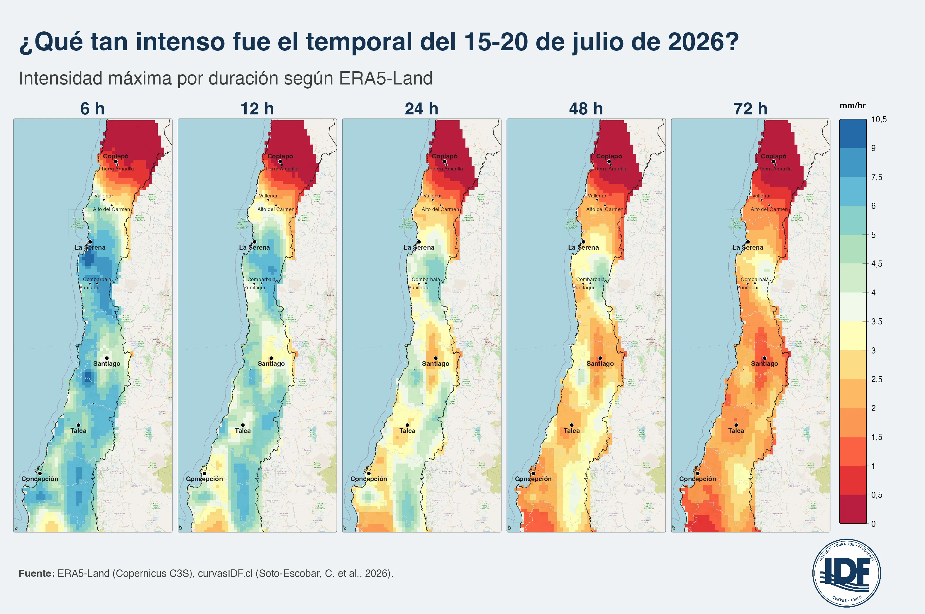
Figure 1. Estimated maximum mean intensity during the 15-20 July 2026 storm, in millimetres per hour, for moving windows of 6, 12, 24, 48 and 72 hours. Each panel shows, for each grid cell, the continuous window of its respective duration with the largest accumulated precipitation during the episode, expressed as mean intensity. The scale is common to all five panels, so intensities can be compared directly across durations. Hourly data from the preliminary ERA5-Land product (Copernicus C3S), bias-corrected.
Figure 2 presents the same maximum mean intensity field, but focused on Atacama and Coquimbo. For the 6-hour window, the strongest spatial contrast is observed: the interior of Atacama, particularly between Copiapó and Tierra Amarilla, has intensities below 0.5 mm/h, while coastal and inland sectors of Coquimbo, between La Serena and the Limarí Valley, reach values up to about 10.5 mm/h.
As the duration considered increases, this contrast weakens. In the 72-hour window, inland Atacama remains below 0.5 mm/h, while the Vallenar sector shows mean intensities of about 1-2 mm/h. By contrast, sectors near La Serena and Combarbalá, which were among the 6-hour maxima, show mean intensities below about 4 mm/h when the wettest 72 hours are considered. This reduction does not imply a decrease in precipitated volume; it is the effect of averaging accumulated precipitation over a much longer time window.
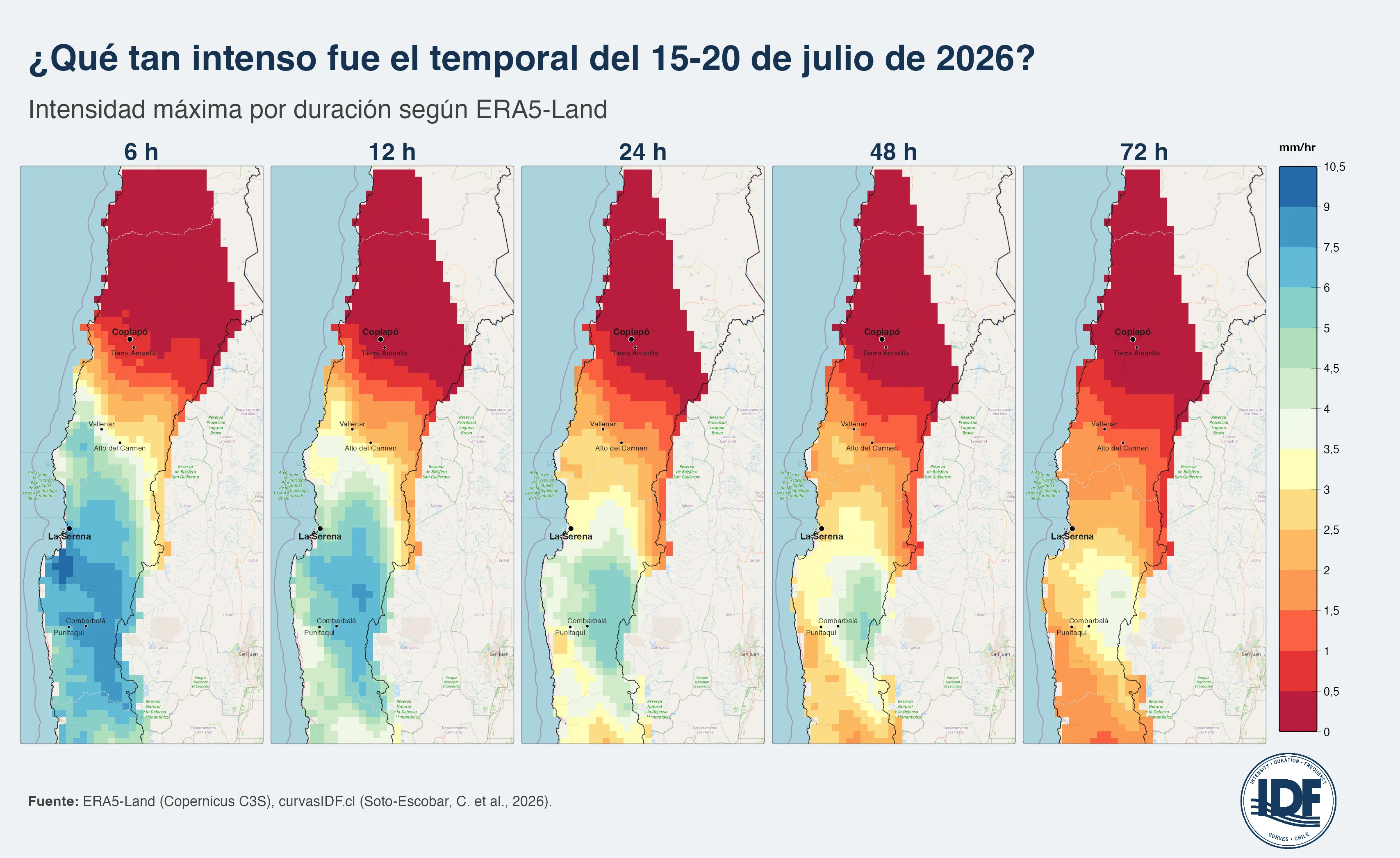
Figure 2. Maximum mean intensity of the storm, in millimetres per hour, for moving windows of 6, 12, 24, 48 and 72 hours, focused on Atacama and Coquimbo. The scale, colour palette and data source are the same as in Figure 1. Hourly data from the preliminary ERA5-Land product (Copernicus C3S), bias-corrected.
Figure 3 presents the maximum accumulated precipitation associated with each analysed duration. These values correspond to the product of the maximum mean intensity shown in Figure 1 and the duration of the corresponding time window. The five panels therefore represent the maximum amount of precipitation accumulated during any continuous interval of 6, 12, 24, 48 or 72 hours within the episode.
The range of accumulations increases substantially with duration, from approximately 61 mm for 6 hours to close to 288 mm for 72 hours. For this reason, the colour-scale intervals widen progressively between classes; using uniform intervals would compress the values associated with the shorter durations and make their spatial interpretation more difficult.
This representation makes the importance of event persistence clearer. As duration increases, the core of maximum accumulation shifts from valley sectors toward Andean zones, and the area affected by high accumulations expands. The pattern indicates that the severity of the episode was not determined only by short high-intensity pulses, but also by the persistence of precipitation over prolonged periods.
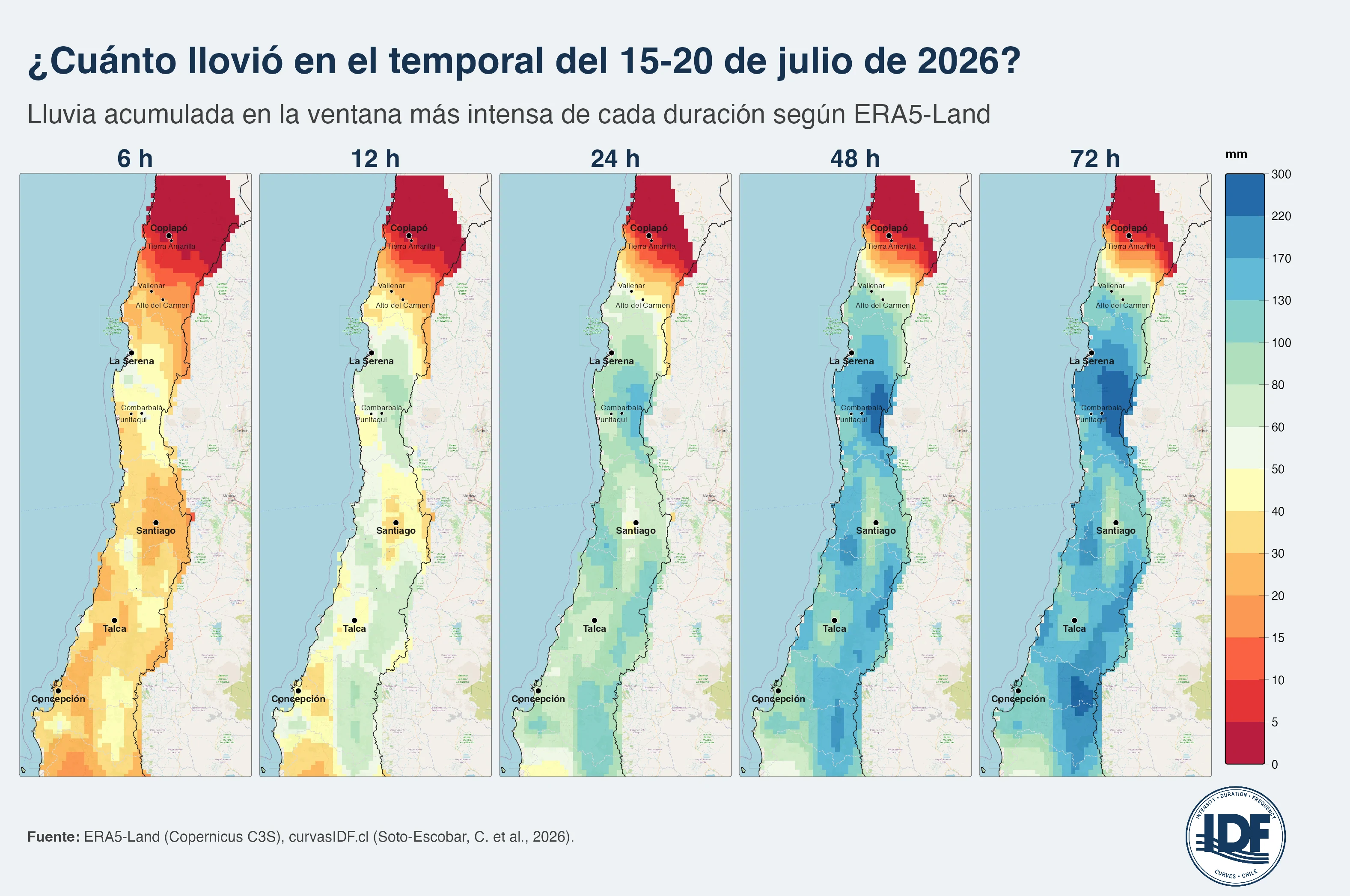
Figure 3. Maximum accumulated precipitation, in millimetres, within the wettest window of each duration. Values are obtained by multiplying the maximum mean intensity in Figure 1 by the corresponding duration. They do not represent total precipitation over the six-day event, but the maximum accumulation recorded in any continuous 6, 12, 24, 48 or 72 hour window within the episode. The start time of the maximum window can vary between grid cells. Scale intervals widen progressively because the accumulation range increases from approximately 61 to 288 mm. Hourly data from the preliminary ERA5-Land product (Copernicus C3S), bias-corrected.
Figure 4 shows the same maximum accumulations focused on Atacama and Coquimbo. Inland Atacama remains below approximately 5 mm for all five durations considered. Toward the south, by contrast, accumulations increase both spatially and with the window duration. For 24 hours, sectors near La Serena and the Limarí Valley reach about 60-100 mm. In the 72-hour window, broad sectors between La Serena, Combarbalá and Punitaqui show accumulations on the order of 220-300 mm, close to the regional maximum of approximately 288 mm.
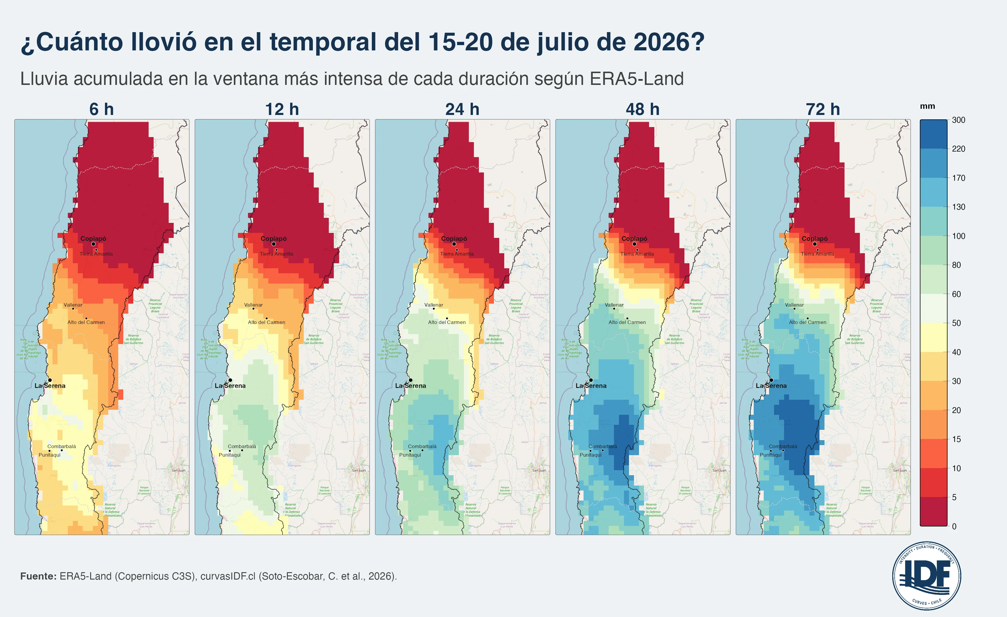
Figure 4. Maximum accumulated precipitation, in millimetres, within the wettest time window of each duration, focused on Atacama and Coquimbo. The scale, colour palette and data source are the same as in Figure 3.
It is important to emphasize that Figures 3 and 4 do not represent total accumulated precipitation during the six days of the storm. Each cell shows the maximum accumulation within a fixed-duration time window, whose start time can differ spatially. Therefore, the maximum windows of two neighbouring cells do not necessarily correspond to the same chronological interval.
The total event precipitation is shown later, in the left panel of Figure 9. Maintaining this distinction is fundamental: although both products are expressed as accumulated precipitation, they answer different hydrometeorological questions. Figures 3 and 4 quantify maximum accumulated precipitation for specific durations, while Figure 9 represents the total volume precipitated during the complete episode.
4. Where was this event “unprecedented”?
When the question changes from how much it rained to how exceptional the precipitation was relative to local climatology, the spatial pattern changes substantially. The main core of exceptionality appears in the interior of Huasco Province, in Atacama, near 28° S. The largest estimated return periods for the 24-, 48- and 72-hour windows are concentrated there. This is not the zone where ERA5-Land estimated the largest absolute intensities or accumulations, but the one where the precipitation observed during the episode departed most strongly from the climatological distribution of extremes used as a reference.
Coquimbo is the second main focus and the region where this exceptional signal reached the largest spatial extent. For the 48-hour window, 47 % of its area had estimated return periods above 500 years; for 72 hours, this proportion increased to 64 %. Between Valparaíso, the Metropolitan Region and O’Higgins, by contrast, a more moderate and spatially localized signal predominated. In these regions, the 48-hour window was more exceptional than the 72-hour window in several sectors. This is a reminder that return period does not have to increase monotonically with duration: each duration has its own annual-maximum distribution and therefore a different extreme climatology. In Maule and Ñuble, comparatively low return periods predominated, although some localized higher-exceptionality cores persisted.
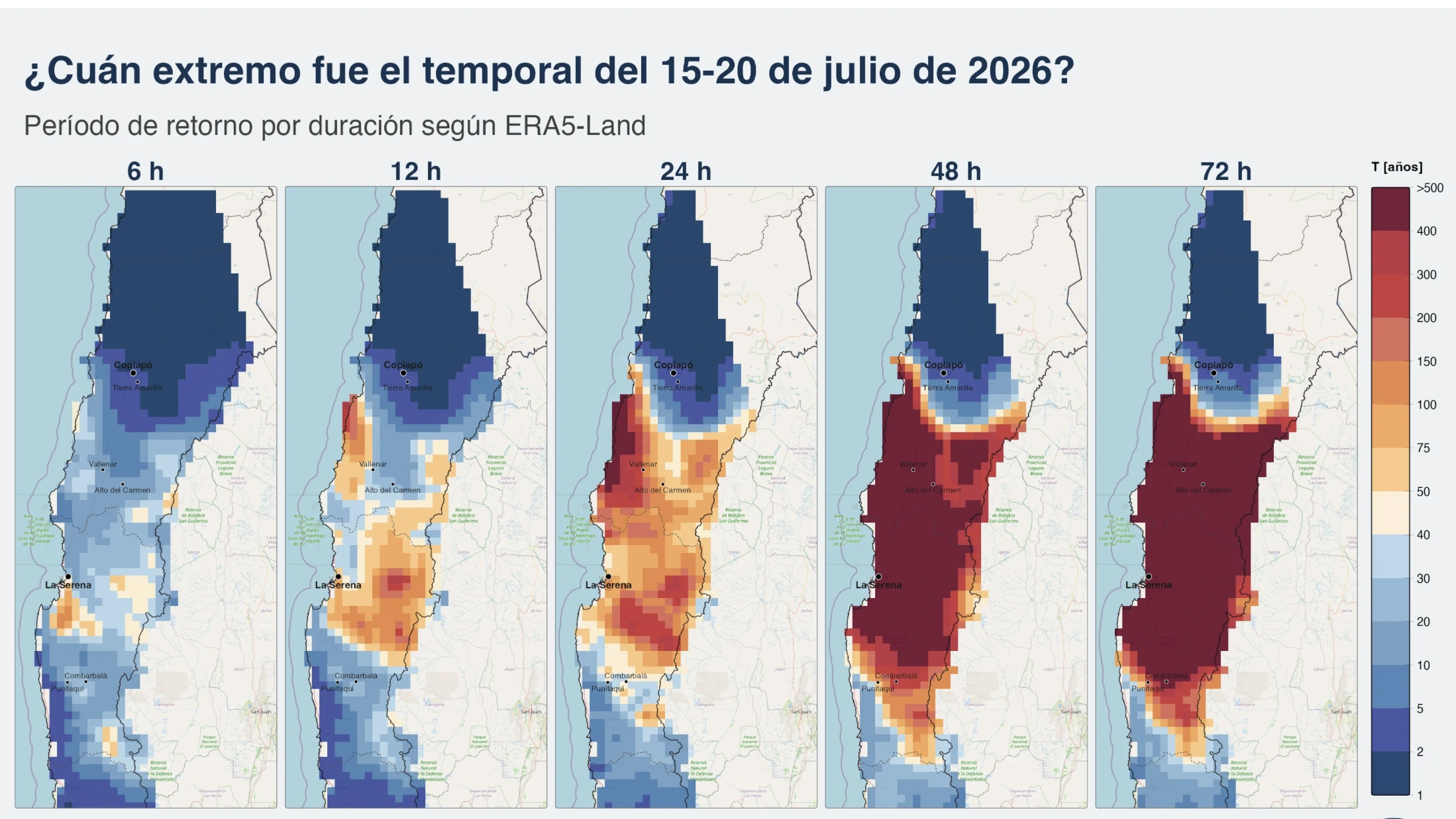
Figure 5 shows the estimated return period for the five analysed durations. The scale ends in an open class of “more than 500 years”: all values placed above that threshold by the probabilistic model are grouped in a single class. This decision is deliberate. The curves were fitted to 41 annual maxima for the 1981-2021 period, so estimates of several hundred years imply extrapolation far beyond the effective record length. Consequently, it is not statistically justified to interpret differences between, for example, return periods of 600, 1,000 or several thousand years as precise estimates.
The maps show that the area associated with very high return periods increases markedly in the 48- and 72-hour windows. This behaviour indicates that, especially in the arid north, the persistence of precipitation for two or three days was climatologically more exceptional than the maxima associated with shorter pulses. The main diagnostic value of these results is therefore not to interpret the extreme return periods literally, but to identify where the episode was far above the annual-maximum climatology used for the fit and where statistical extrapolation, and therefore uncertainty, becomes dominant. For the 72-hour window, 20.5 % of the analysed continental area is classified above the 500-year threshold.
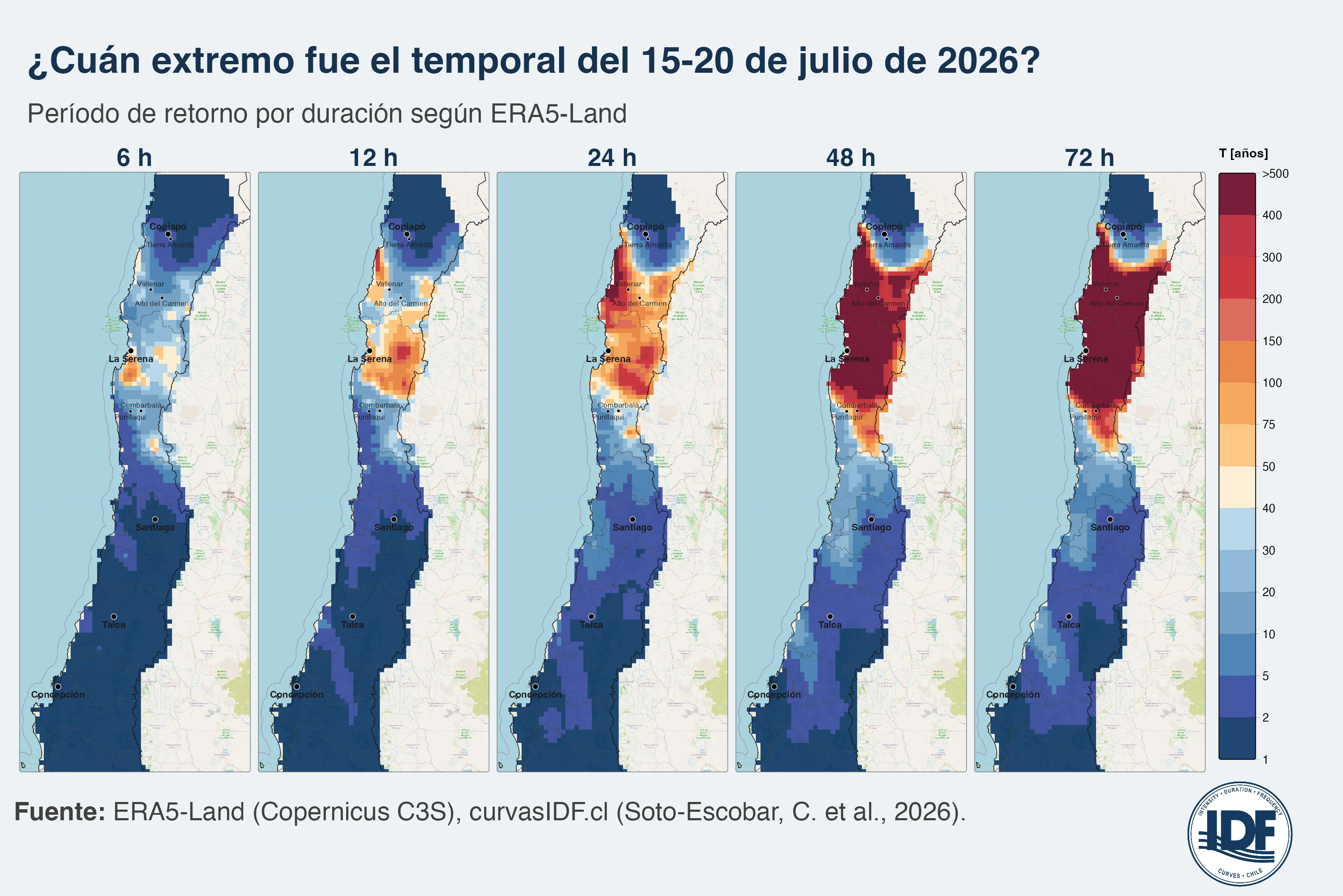
Figure 5. Estimated return period of the storm, in years, for moving windows of 6, 12, 24, 48 and 72 hours over the analysed continental territory. The scale extends from 1 year to an open class of “more than 500 years”, which groups all estimates above that threshold. Return periods were obtained by fitting a stationary Gumbel distribution to the 41 annual-maximum ERA5-Land series for the 1981-2021 period, following Soto-Escobar et al. (2026). Values in the upper class should be interpreted as indicators of extreme exceptionality, not as precise recurrence estimates.
Figure 6 presents the same analysis focused on Atacama and Coquimbo, where the largest exceptional signal of the storm was concentrated. This zoom makes it possible to observe how the spatial pattern evolves with duration. For 24 hours, the upper class of more than 500 years still appears as relatively isolated cores, mainly in inland Huasco and in sectors near La Serena, surrounded by areas with return periods on the order of 50 to 150 years.
For 48 hours, these cores expand and begin to form a band of high exceptionality between the surroundings of Copiapó and the Limarí Valley. In the 72-hour window, the upper class extends over much of the interior of both regions and continues southward to sectors near Combarbalá and Punitaqui, where it transitions toward return periods on the order of 100 to 400 years. South of Punitaqui, lower values again predominate, generally below 20 years for all five durations considered.
This pattern confirms a central feature of the episode: the largest anomalies relative to local climatology do not necessarily coincide with the zones of greatest absolute precipitation. In Atacama, comparatively modest accumulations can correspond to very high return periods because of the historically low frequency and intensity of prolonged precipitation in this region.
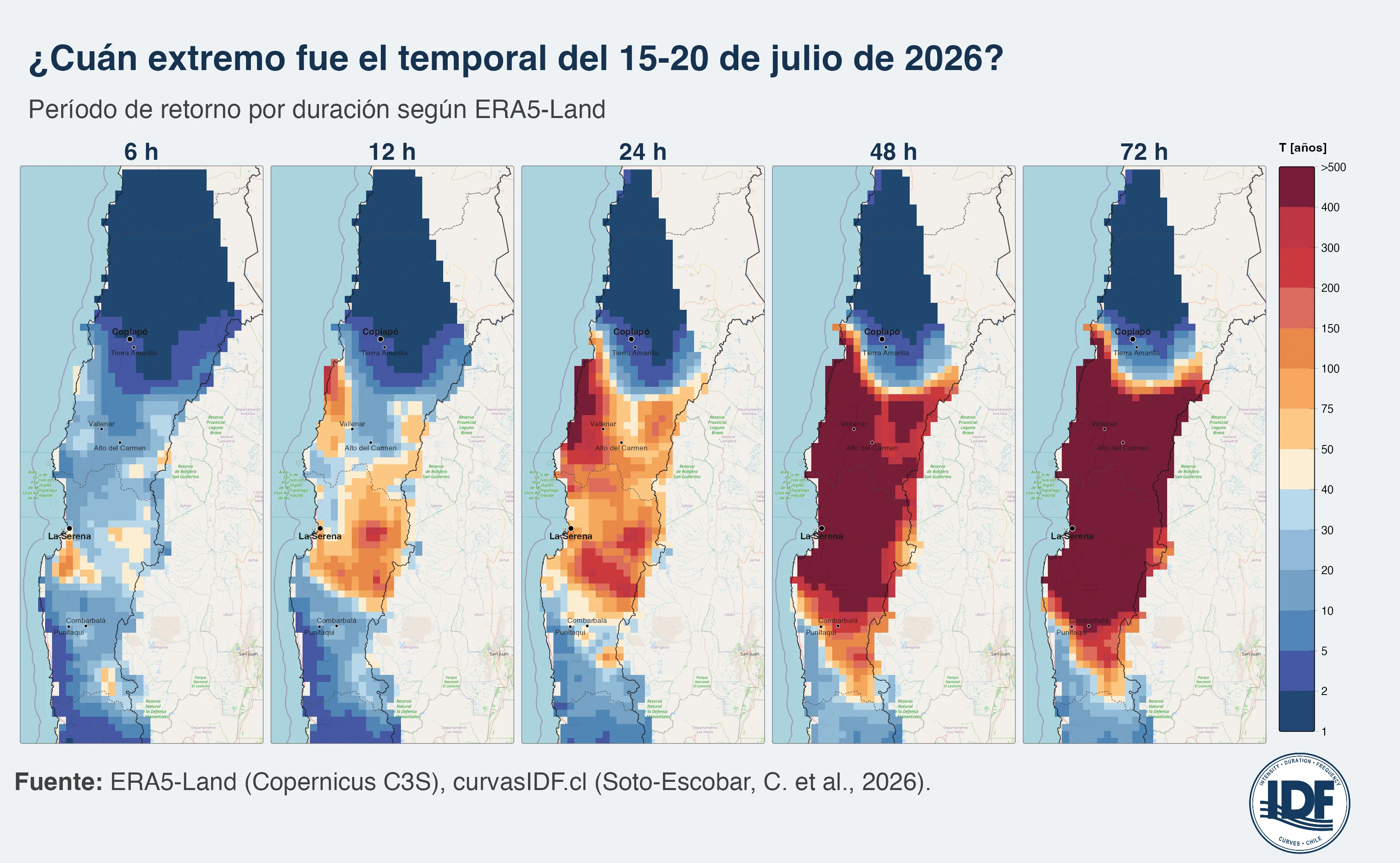
Figure 6. Estimated return period of the storm, in years, for moving windows of 6, 12, 24, 48 and 72 hours, focused on Atacama and Coquimbo, where the largest exceptional signal of the episode was concentrated. The same scale, data source and statistical methodology as in Figure 5 are used. The “more than 500 years” class should be interpreted as an open class of extreme exceptionality, given the uncertainty inherent in extrapolating a distribution fitted to 41 annual maxima.
5. What uncertainty do these estimates have?
The previous maps show the return periods obtained from the probabilistic fit, but the largest T values should not be interpreted as directly observable frequencies or as estimates that are equally precise across their full range. The case of Vallenar illustrates this difference. For a duration of 24 hours, the 2026 storm reached a mean intensity of 2.3 mm/h and corresponded to the second-highest value among the 41 annual maxima analysed, only below the 1997 maximum. Using an empirical plotting position based exclusively on the ordering of the data, the second maximum in a 41-year sample corresponds to a return period of approximately 21 years. However, the fitted Gumbel distribution assigns the same intensity a return period of approximately 235 years.
This difference is not a calculation inconsistency: it reflects that both estimates respond to different concepts. The empirical return period depends mainly on the position that the event occupies within the observed sample, whereas the parametric return period is obtained from the exceedance probability assigned by the fitted distribution. The two values can therefore differ substantially, especially when the sample size is limited and the event lies in the tail of the distribution.
This situation is particularly relevant in arid regions such as Atacama, where annual-maximum series contain many years with very small precipitation and a few considerably larger episodes. The fitted location and scale of the Gumbel distribution then define a tail in which relatively small intensity increases can translate into large variations in return period. In this context, a high T value mainly expresses that the event lies far from the probabilistic behaviour characteristic of local annual maxima; it does not imply that there is enough observational evidence to estimate a recurrence of several hundred years precisely.
For this reason, parametric return periods should be interpreted together with the event’s position within the observed record and with its statistical uncertainty. The record indicates how many comparable observations actually exist in the 41 available years; the model allows extrapolation beyond that range under the assumptions of the adopted distribution. Both readings are complementary, but their degree of observational support is different.
Figure 7 compares the intensity-duration-frequency (IDF) curves with the storm trajectory at three representative locations: Vallenar, the Limarí Valley and Punitaqui. In each panel, the warm-coloured curves represent return periods between 2 and 500 years, while the eleven blue points describe the event’s maximum mean intensities for durations from 1 to 72 hours.
The event trajectory shows why duration is decisive for evaluating exceptionality. In Vallenar, intensities for durations up to approximately 12 hours remain within the range associated with T <= 25 years, but the event curve progressively separates from the IDF curves as duration increases. This indicates that the most exceptional feature of the storm in this sector was not a short pulse of high intensity, but the persistence of precipitation for one or several days. In Punitaqui, the return period also increases with duration, although the trajectory remains much closer to the range supported by the reference curves. The value of the plot lies precisely in replacing the reading of a single T with the complete trajectory of the episode across multiple durations.
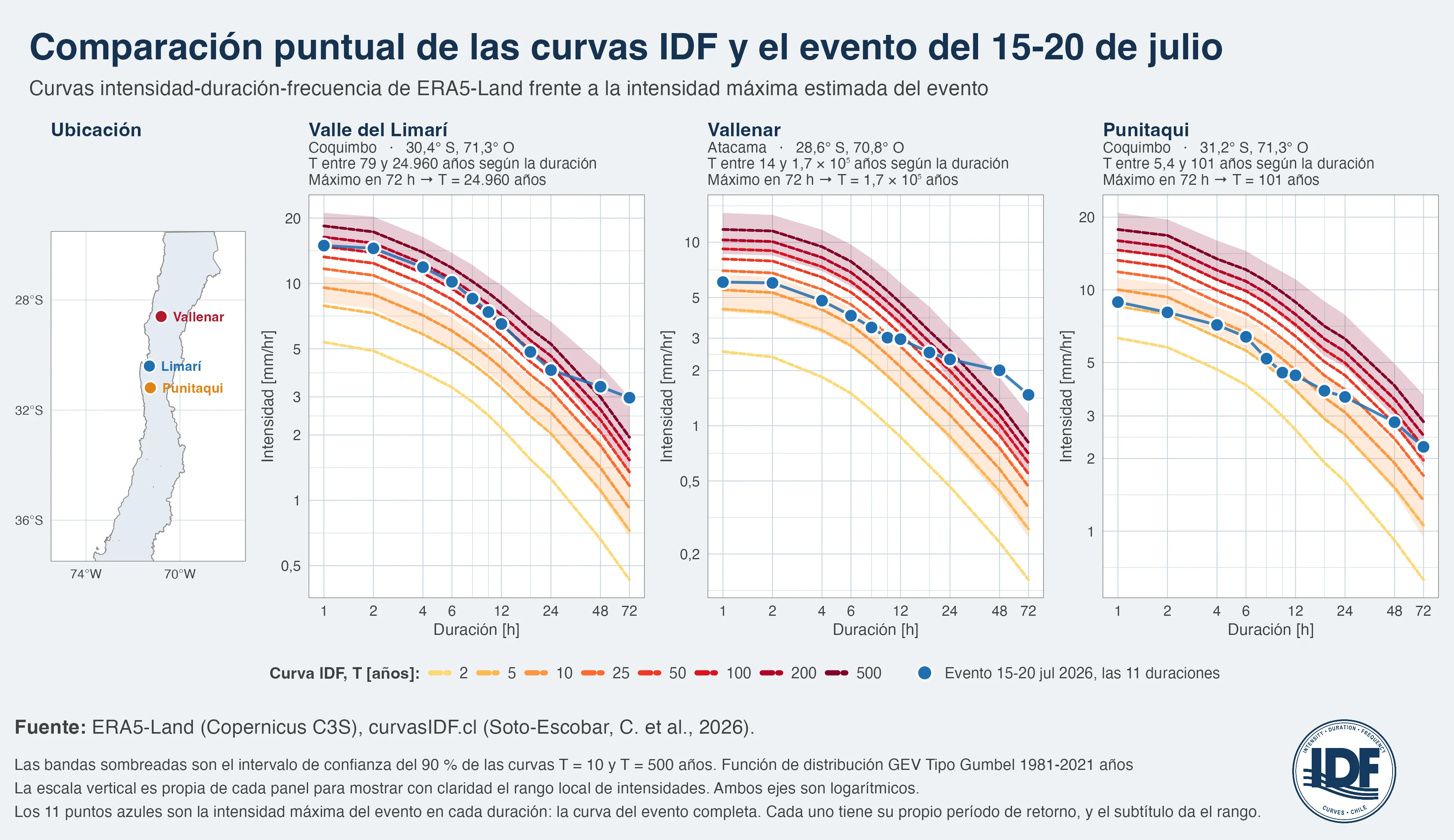
Figure 7. ERA5-Land intensity-duration-frequency curves compared with the estimated maximum mean intensities during the storm, in three representative cells: Vallenar (Atacama), the Limarí Valley (Coquimbo) and Punitaqui (Coquimbo). Warm-coloured lines correspond to IDF curves for return periods of 2, 5, 10, 25, 50, 100, 200 and 500 years. The eleven connected blue points represent the event’s maximum mean intensities for the analysed durations between 1 and 72 hours. Shaded bands show 90 % confidence intervals for the 10- and 500-year curves, obtained by bootstrap resampling. Both axes are shown on logarithmic scales and each panel uses its own vertical scale to properly represent the local intensity range.
To quantify fitting uncertainty, we repeated the Gumbel estimation 1,000 times using bootstrap resampling with replacement of the 41 annual maxima. This procedure evaluates how much the estimates vary because of the limited length of the available series.
The results show that uncertainty increases rapidly when the event intensity lies outside, or very close to the upper end of, the observed range. In Vallenar, for a 48-hour duration, even the lower percentile of the 90 % bootstrap interval corresponds to an estimated return period of approximately 963 years. This result indicates that, within the adopted statistical model and the realizations generated by resampling, the event intensity remains far from the annual-maximum climatology used for the fit.
However, this result should not be interpreted as evidence that the “real” return period is at least 963 years. On the contrary, when the entire bootstrap distribution shifts toward return periods far above the record length, the result indicates that extrapolation dominates the estimate. In that regime, the analysis supports the statement that the episode was extraordinarily infrequent relative to the climate represented by ERA5-Land during 1981-2021 more robustly than it supports assigning a precise recurrence frequency. The farther T moves away from the 41 years of information used to fit the model, the greater the caution required in its numerical interpretation.
Figure 8 makes it possible to examine this situation directly. The grid contains nine panels: rows correspond to Vallenar, the Limarí Valley and Punitaqui, and columns to durations of 24, 48 and 72 hours. Each panel shows the 41 annual maxima, the fitted Gumbel distribution, its uncertainty interval and the position occupied by the 2026 storm. The vertical line indicates the maximum recorded during 1981-2021; to the right of this limit, any estimate necessarily depends on extrapolation of the probabilistic model.
The comparison between the three locations helps evaluate how strongly the return period is supported by observations. In Punitaqui, where historical maxima approach the range reached by the storm, the 2026 point remains relatively close to the observation cloud and the fitted return periods remain comparatively close to the available information range: approximately 18 years for 24 hours and 101 years for 72 hours. In Vallenar, by contrast, the 2026 event clearly separates from the historical maxima for the longer durations. In these cases, the position of the event relative to the edge of the record provides an immediate visual indication of how much the estimated return period depends on extrapolation.
This comparison allows each T value to be accompanied by the evidence supporting it and distinguishes two conceptually different situations: cases in which the event magnitude is within or close to the observed range, where the estimate is relatively supported by the record, and cases in which the event clearly lies outside it, where return period depends mainly on assumptions about tail behaviour.
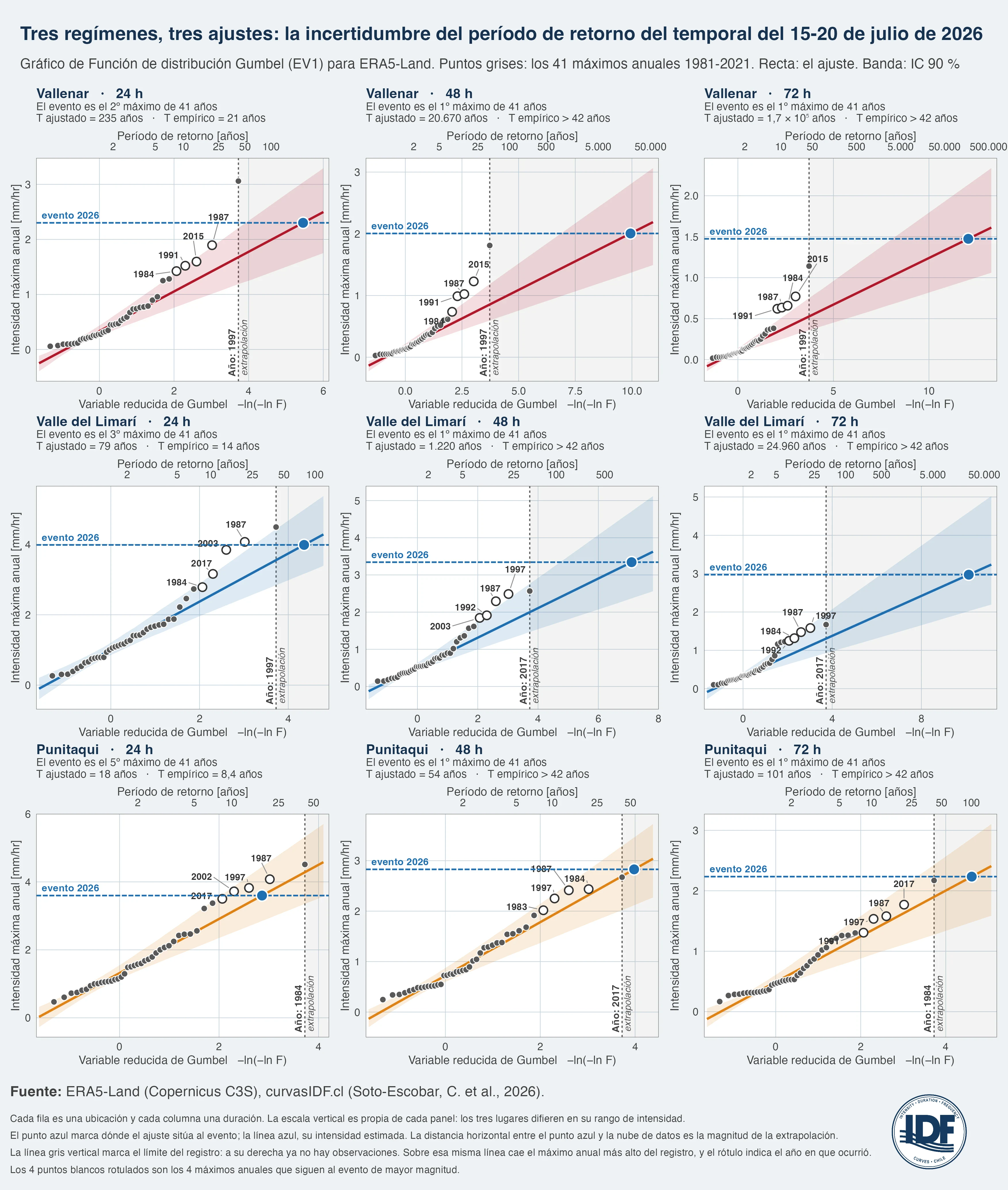
Figure 8. Gumbel probability plots. Rows correspond to Vallenar, the Limarí Valley and Punitaqui, and columns to durations of 24, 48 and 72 hours. Grey points represent the 41 annual maxima of ERA5-Land during 1981-2021. The four labelled white points correspond to the largest years after the historical maximum, while the blue point represents the 2026 storm. The line is the Gumbel fit and the shaded band is its 90 % confidence interval, estimated by bootstrap resampling. The grey vertical line indicates the maximum observed during 1981-2021, identified by its year of occurrence; values to its right are outside the observed range and therefore correspond to extrapolations of the probabilistic model. Each panel uses its own vertical scale.
6. How did it affect us? Rainfall chronology and emergencies
The storm showed a marked south-to-north displacement. Precipitation was initially concentrated in Maule and Biobío on 15 and 16 July, reached central Chile on 17 July and later intensified over Coquimbo and Atacama on 19 and 20 July. The estimated hourly maximum within the analysed area was located near 30.6° S on 19 July at 21:00, with an intensity of approximately 11.2 mm/h.
During the six-day episode, the Ministry of Public Works (MOP) recorded 649 infrastructure-related emergency reports within the study area: 240 classified as minor, 255 as moderate, 135 as severe and 19 as very severe. The Directorate of Roads accounted for 461 records, equivalent to 71 % of the total. Regionally, Coquimbo accumulated 311 reports and Atacama 110; together, both regions concentrated approximately 65 % of the recorded emergencies. The daily maximum occurred on 20 July, when 238 reports were counted, coinciding with the phase in which the most important precipitation had shifted toward the north of the analysed territory.
Figure 9 integrates three complementary perspectives of the episode: total accumulated precipitation, the spatial distribution and severity of MOP reports, and the joint hourly evolution of precipitation and emergencies as a function of latitude. In the right-hand panel, the horizontal axis represents time and the vertical axis latitude; colours indicate the estimated maximum hourly intensity for each latitudinal band and points represent emergency reports.
To build this diagram, we used, for each latitudinal band and hour, the maximum precipitation intensity across all continental longitudes, not the average. This choice preserves the signal of intense cores that could be attenuated by averaging coastal, valley and mountain sectors at the same time. The result clearly shows the propagation of the precipitation band from south to north and a concentration of emergency reports in space-time bands close to the passage of the system. Figure 9 therefore jointly reconstructs the meteorological evolution of the episode and the timing of its infrastructure impacts.
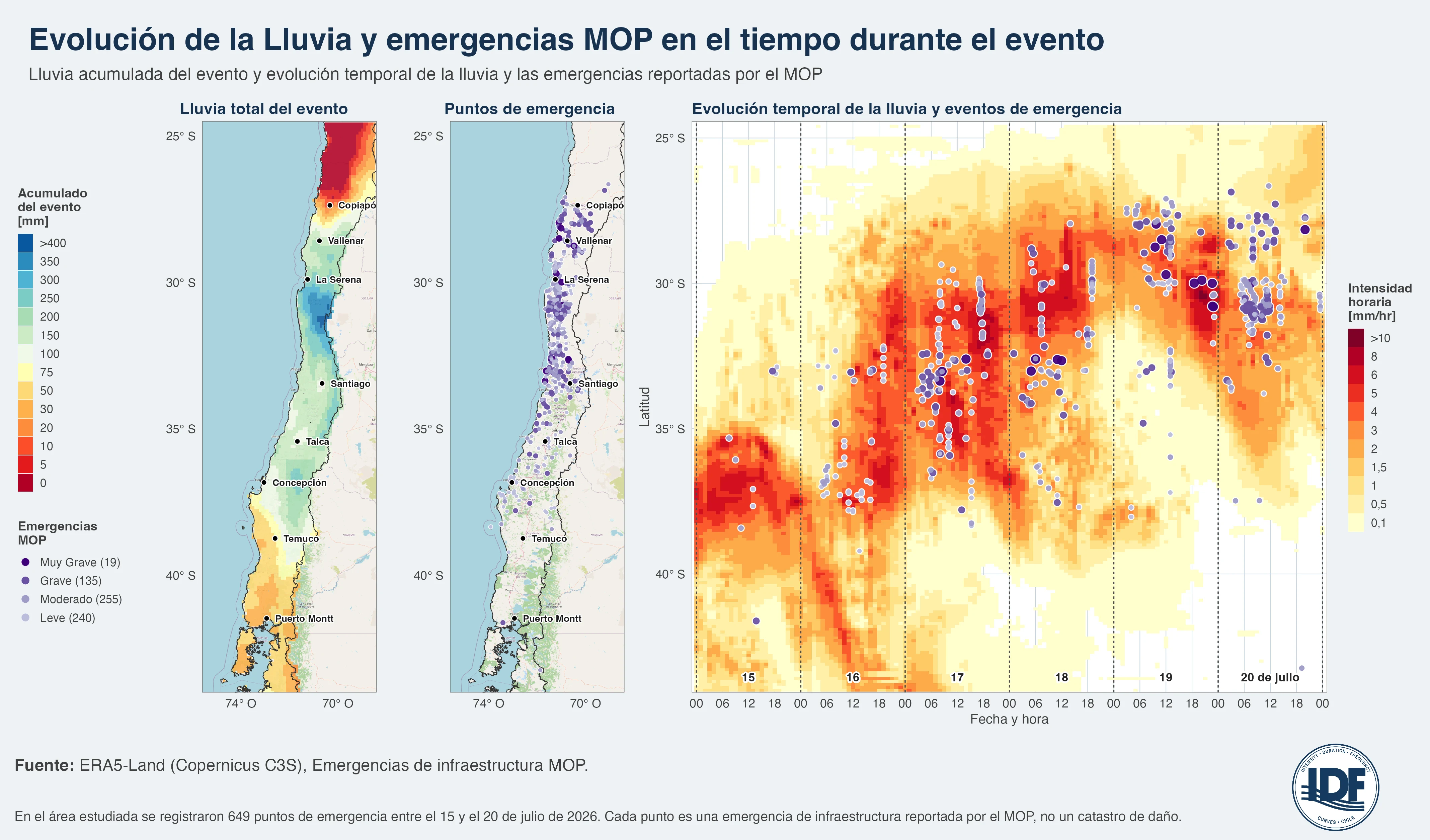
Figure 9. Evolution of precipitation and infrastructure emergencies during the storm, represented in three complementary views. Left: total accumulated precipitation during the event, in millimetres. Centre: location of the 649 infrastructure emergency reports recorded by MOP between 15 and 20 July 2026, with symbol size and colour representing severity level. Right: joint evolution of both variables: the horizontal axis represents date and time in continental Chile local time, the vertical axis latitude, and colour the maximum estimated hourly intensity within each latitudinal band, calculated across all continental longitudes and not as a zonal average. Points correspond to the same emergency reports, located by time and latitude. Sources: ERA5-Land (Copernicus C3S) and MOP infrastructure emergency records.
The space-time evolution suggests a close correspondence between the displacement of precipitation and the sequence of infrastructure emergencies. Reports tend to appear in latitudinal bands and periods close to the passage of the main precipitation cores, while severe and very severe events are concentrated especially in Coquimbo and Atacama, the same regions where the episode combined high persistence with strong exceptionality relative to local climatology.
This correspondence does not, by itself, imply a direct causal relationship between hourly intensity and each individual emergency. Infrastructure response also depends on antecedent and accumulated precipitation, catchment size and time of concentration, previous soil moisture, geomorphological and drainage characteristics, the state of infrastructure maintenance and territorial exposure. In addition, the registered time of an emergency can differ from the moment when the damage physically occurred.
This last point is particularly important when interpreting temporal lags. In the band between 31° and 30° S, the median report time occurred 9.2 hours after the hourly precipitation maximum. This lag is compatible with both hydrological catchment response times and the interval required to detect, verify, survey and communicate an emergency from the field. Therefore, the 9.2 hours should not be interpreted directly as a catchment response time, but as the combined result of hydrological and operational processes.
The results of the previous sections add another important dimension for interpreting these impacts: in Coquimbo and Atacama, durations of 48 and 72 hours were climatologically more exceptional than short-duration pulses. For catchments and infrastructure whose response integrates precipitation over several hours or days, this persistence can be as important as the maximum hourly intensity. The exact relationship between critical duration, hydrological response and failure mechanism, however, depends on the scale and specific characteristics of each system.
The human and material balance confirms the magnitude of the episode. According to the new SENAPRED balance reported by CNN Chile , the frontal system caused 13 deaths, 18 missing people, 18,254 affected/displaced people, more than 1,700 people in shelters and 45,108 isolated people, mainly in Coquimbo and Atacama. In housing, the same balance recorded 1,679 destroyed homes, 8,492 with major damage, 34,741 with minor damage and 552 under assessment.
For public infrastructure, MOP estimated on 27 July a requirement of US$400-500 million to recover damage in Coquimbo and Huasco Province, an amount that could reach US$700 million when previously accumulated liabilities in roads, water resources and telecommunications are included. These values correspond to a preliminary estimate of reconstruction needs, so they should not be interpreted as a direct quantification or as exclusively attributable to the damage caused by this storm.
In the mining sector, the Coordinadora de Trabajadores de la Minería (CTMIN) projected an aggregate economic impact of US$120-235 million for the period between 13 and 26 July across five regions. The estimate integrates production losses, operational overruns, emergency logistics and indirect effects, and depends on assumptions about extraction levels and copper prices. It should therefore be interpreted as a preliminary sectoral estimate, not as a direct observational measurement of economic losses caused exclusively by the 15-20 July episode.
7. Uneven hydrological and sectoral effects
The storm also produced important changes in surface water storage. Between the DGA hydrological bulletins of 13 and 27 July, the volume stored in the 25 monitored reservoirs increased from 3,713 to 5,215 million cubic metres. As a group, these reservoirs were 21.1 % below the volume recorded in 2025 before the event and, after the storm, stood 10.8 % above that reference value.
The increase was especially marked in Coquimbo. La Paloma reservoir rose from 35.9 to 202.2 million cubic metres, Cogotí from 15.2 to 123.1 million cubic metres, and Recoleta reached storage capacity. These variations show that the same hydrometeorological episode can simultaneously generate adverse impacts and benefits for water availability. However, the increase observed between the two bulletins should not be interpreted as a direct conversion of storm precipitation into storage: the response of each reservoir depends on catchment inflows, concentration and routing times, antecedent conditions, withdrawals and operating rules during the period considered.
In the agricultural sector, SNA reported on 20 July that, up to that point, it did not observe significant impacts on production, although it did report important damage to roads, bridges, irrigation systems, electricity networks and rural connectivity. The estimate of up to US$200 million circulated during those days corresponded to preliminary third-party estimates, not to an economic assessment prepared directly by SNA.
These results illustrate the spatially and sectorally heterogeneous nature of the episode. Increased water storage and continuity in part of agricultural production coexisted with severe damage to infrastructure, connectivity and irrigation systems. Positive effects on water availability therefore do not offset or relativize the losses: benefits and damages occurred in different places, time scales, economic activities and communities.
8. What does this analysis reveal?
The most consistent result is that the exceptionality of the storm was mainly associated with its duration and persistence, rather than with extraordinary hourly intensities. The fraction of the analysed continental area with estimated return periods above 500 years is zero for the 6- and 12-hour windows and reaches only 0.8 % for 24 hours. However, it increases abruptly to 14.2 % for 48 hours and 20.5 % for 72 hours. In other words, the most statistically exceptional feature of the episode was not an isolated hourly pulse, but the persistence of precipitation for two to three days over arid and semi-arid sectors.
This result has a direct hydrological consequence: critical duration depends on both the territory and the system being analysed. In Atacama and Coquimbo, the greatest exceptionality is observed for the 72-hour window. Between Valparaíso, the Metropolitan Region and O’Higgins, by contrast, the most anomalous signal is concentrated preferentially in 48 hours and decreases when the analysis is extended to 72 hours. This occurs because each duration has its own annual-maximum distribution: the return period of a precipitation event does not necessarily increase monotonically with duration.
For this reason, the evaluation of hydraulic infrastructure should not be based simply on the longest available duration, but on the time scales relevant to its hydrological and hydraulic response. An urban drainage network may be controlled by intense precipitation lasting minutes or hours, while a larger catchment, a river system or a reservoir may respond mainly to accumulations over several tens of hours or several days.
The analysis also shows that absolute magnitude and climatological exceptionality have different spatial patterns. The largest estimated value for the 6-hour window was located in the Limarí Valley, with approximately 61 mm accumulated, equivalent to a mean intensity of 10.2 mm/h. The largest return periods, by contrast, were located several degrees of latitude farther north, mainly in the interior of Huasco Province, where absolute intensities were considerably lower.
This difference is fundamental for interpreting hydrometeorological extremes: the same amount of precipitation can represent very different probabilistic situations depending on local climatology. Similarly, relatively nearby places can record different accumulations and, at the same time, occupy very different positions within their respective extreme-value distributions. For the 72-hour window, for example, the Limarí Valley accumulated approximately 214 mm, while Punitaqui, about 90 km farther south, reached close to 160 mm.
Finally, the spatial distribution of exceptionality shows a notable, though not necessarily causal, correspondence with the distribution of infrastructure emergencies. Coquimbo and Atacama concentrated 65 % of the reports recorded by MOP and were also the two regions where long-duration precipitation reached the largest return periods. The daily maximum number of reports also occurred on 20 July, when the main precipitation band had shifted toward the northern part of the study area.
This space-time coincidence is consistent with a relationship between rainfall persistence and impacts, but it does not allow each emergency to be attributed exclusively to rainfall magnitude or exceptionality. Damage also depends on the hydrological response of each catchment, antecedent conditions, exposure, vulnerability and the prior state of infrastructure.
9. How can we be better prepared?
The storm did not have the same statistical character across the affected territory. In Atacama and Coquimbo, its main singularity was precipitation persistence over 48 and 72 hours. Between Valparaíso and O’Higgins, the greatest exceptionality appeared mainly in the 48-hour window. In Maule and Ñuble, by contrast, much of the precipitation remained within considerably lower recurrence ranges. This heterogeneity prevents the episode from being adequately characterized by a single value of intensity, accumulation or return period.
The same consideration is fundamental for hydraulic-infrastructure design and evaluation. There is no universal critical duration for the whole territory or for all types of works. Each system should be analysed using precipitation associated with its location, spatial scale and the time interval that controls its response. The relevant duration for an urban culvert, for example, can be very different from the duration governing the design flow of a river or the operation of a reservoir spillway.
For this purpose we developed curvasIDF.cl , an open platform for spatial characterization of extreme precipitation and analysis of intensity-duration-frequency curves in Chile. The tool allows users to consult IDF curves for any point in the territory covered by the available products and explore different combinations of duration and return period using the same methodological basis applied in this analysis.
IDF curves are a fundamental tool for relating intensity, duration and frequency of extreme precipitation. Their use in design should, however, consider the resolution and nature of the source data, the uncertainty associated with estimating extremes and the statistical assumptions of the adopted model, especially when extrapolating toward return periods far greater than the length of the available record.
Tool:
Article:
- Soto-Escobar, C., Zambrano-Bigiarini, M., Tolorza, V., and Garreaud, R.: Developing Intensity-Duration-Frequency (IDF) curves using sub-daily gridded and in situ datasets: characterising precipitation extremes in a drying climate, Hydrol. Earth Syst. Sci., 30, 91-117, https://doi.org/10.5194/hess-30-91-2026
Sources
- Soto-Escobar, C., Zambrano-Bigiarini, M., Tolorza, V., and Garreaud, R. (2026). Developing Intensity-Duration-Frequency (IDF) curves using sub-daily gridded and in situ datasets: characterising precipitation extremes in a drying climate . Hydrology and Earth System Sciences, 30, 91-117.
- SENAPRED’s new frontal-system balance reported by CNN Chile: 13 deaths, 18 missing people, 18,254 affected/displaced people, more than 1,700 people in shelters, 45,108 isolated people and damaged housing .
- MOP preliminary reconstruction estimate as of 27 July 2026, reported by La Tercera: up to US$700 million for Atacama and Coquimbo .
- Dirección General de Aguas (DGA), hydrological bulletins .
- Sociedad Nacional de Agricultura, 20 July 2026 frontal-system balance .
- Coordinadora de Trabajadores de la Minería (CTMIN), report published by Acero y Roca: storm impacts on Chilean mining .
- CR2 (2026). The 15-20 July 2026 extreme event in the context of a developing El Niño .
- Meteored (2026). El Niño and a category 4 atmospheric river: keys to the historic storm that hit Chile .
- Minvu (2026). Chapter 5. Urban stormwater design .
- MOP (2025). Manual de Carreteras Chile - 2025 edition .